Inconsequential Musings

Contributing LU decomposition code to the Sympy project got me to thinking about backward error analysis of linear systems. A computer algebra system such as Sympy can compute the exact solution to a system of equations, in contrast to an approximate solution computed by an algorithm that employs floating point arithmetic. With an approximate and exact solution in hand, we can use a computer algebra system to compute the exact error in the solutions, and the backward error in the right hand sides. A simple experiment in Sympy revealed that my understanding of the relationship between backward and forward error for an ill-conditioned linear system was incomplete. It’s my hope that someone will find my misconception enlightening.

Let \(\mathcal{A}\) denote an algorithm that solves the linear system \(Ax=b\). If the algorithm runs on a machine that performs its computation in floating point arithmetic, then \(\mathcal{A}\) typically will not produce the exact solution \(x\). Rather, it produces an approximate solution \(\bar{x}\)
\[
\bar{x} \equiv \mathcal{A}(A, b)
\]
where the residual \(b-A\bar{x}\) is typically nonzero. Naturally, anyone who uses \(\mathcal{A}\) to solve a system of equations would like an upper bound on the error of the approximate solution it generates. One of the simplest measures of error is the 2-norm relative error, which is what we’ll use to measure solution error:
\[
\text{err}_{\text{soln}} \equiv \frac{\|x-\bar{x}\|_2}{\|x\|_2}
\] A deceptively clever insight of backward error analysis is that if \(A\) is invertible, then the approximate solution \(\bar{x}\) is the exact solution of \(A \bar{x} = \bar{b}\), for some right hand side \(\bar{b}\). It follows from the linearity of \(A\) that the difference between the solutions is related to the difference between the right hand sides by:
\[
x -\bar{x} = A^{-1}(b – \bar{b})
\] The backward error is defined in terms of the two right hand sides as
\[
\text{err}_{\text{back}} \equiv \frac{\|b-\bar{b}\|_2}{\|b\|_2}
\] The 2-norm condition number of \(A\) is defined as \(\kappa_2(A) \equiv \|A\|_2\|A^{-1}\|_2 = \sigma_{\text{max}}/\sigma_{\text{min}}\), where \(\sigma_{\text{max}}\) and \(\sigma_{\text{min}}\) are the largest and smallest singular values of \(A\). Subjectively, a system is said to be ill-conditioned if it has a large condition number. The righthand side perturbation theorem bounds the relative error of the solution by the product of the condition number and the backward error:\[
\frac{\|x-\bar{x}\|_2}{\|x\|_2} \le \kappa_2(A) \frac{\|b-\bar{b}\|_2}{\|b\|_2}
\] Even if the algorithm \(\mathcal{A}\) computes a solution such that the residual \(\|b-\bar{b}\|_2 = \|Ax-A\bar{x}\|_2\) is small, the above bound suggests that the solution error can still can be quite large if the condition number is large. In fact, Golub and Van Loan’s Matrix Computations contains the following similar statement “If\[
A = \sum_{i=1}^n \sigma_i u_i v_i^T = U \Sigma V^T
\] is the SVD of \(A\), then \[
x = A^{-1}b = (U \Sigma V^T)^{-1} b = \sum_{i=1}^n \frac{u_i^T b}{\sigma_i} v_i.
\] This expansion shows that small changes in \(A\) or \(b\) can induce relatively large changes in \(x\) if \(\sigma_n\) is small.” (Matrix Computations, Third edition. Gene H. Golub, Charles F. Van Loan)

In just about every linear algebra textbook I’ve ever studied, the authors first define solution error, condition number, and backward error. Next, they show either by rigorous proof or empirical evidence that widely used algorithms produce an answer that has small backward error. Finally, they then conclude that these algorithms produce accurate solutions when the condition number of the system is not too large. In other words, when the underlying problem is not ill-conditioned, widely used algorithms for solving systems produce accurate results.

When \(A\) is ill-conditioned and dense, experience shows that these same algorithms do not produce accurate solutions. This isn’t surprising given the bound of the righthand side perturbation theorem, and the statement from Golub and Van Loan that “small changes in \(A\) or \(b\) can induce relatively large changes in \(x\) if \(\sigma_n\) is small.” What I found surprising, was that in the numerical experiments I ran with an ill-conditioned \(A\), the solution error and backward error are comparable in magnitude. A description of the numerical experiment follows

In Sympy:

• Convert the entries of \(A\), \(\bar{x}\), and \(b\) to instances of sympy.Rational
• Compute the exact solution \(x\) from \(A\) and \(b\)
• Compute the perturbed right hand side \(\bar{b}\) from \(A\) and \(\bar{x}\)
• Compute the solution relative error \(\frac{\|x-\bar{x}\|_2}{\|x\|_2}\)
• Compute the backward relative error \(\frac{\|b-\bar{b}\|_2}{\|b\|_2}\)
• Compute the ratio of the solution relative error magnitude to the perturbation magnitude of the right hand side: \(\frac{\|x-\bar{x}\|_2}{\|x\|_2}\frac{\|b\|_2}{\|b-\bar{b}\|_2}\). This quantity is also a lower bound on the 2-norm condition number of \(A\)

In this particular experiment, \(A\) was constructed from its singular value decomposition \(A=U \Sigma V^T\) where
\begin{align*}
U=\begin{bmatrix}\cos(\pi/3) & -\sin(\pi/3)\\\sin(\pi/3) & \cos(\pi/3)\end{bmatrix}
&&
\Sigma=\begin{bmatrix}1 & 0\\0 & 2^{-24}\end{bmatrix}
&&
V=\begin{bmatrix}\cos(\pi/4) & -\sin(\pi/4)\\\sin(\pi/4) & \cos(\pi/4)\end{bmatrix}
\end{align*}
The set of right hand sides are evenly distributed around the unit circle.
The condition number of \(A\) is approximately \(2^{24}\) (but not exactly \(2^{24}\) since \(A\) was computed in floating point arithmetic), so \(\kappa_2(A) \approx 1.7 \times 10^8\). The numerical experiments were run on a machine whose machine epsilon is \(\epsilon_{\text{mach}} \approx 2.2 \times 10^{-16}\). Under the optimistic assumption that both algorithms compute solutions whose associated backwards error is less than machine epsilon, the right hand side perturbation theorem guarantees that the forward error is bounded by
\[
\frac{\|x-\bar{x}\|_2}{\|x\|_2} \le \kappa_2(A) \epsilon_{\text{mach}} \approx 10^8 \times 10^{-16} = 10^{-8}
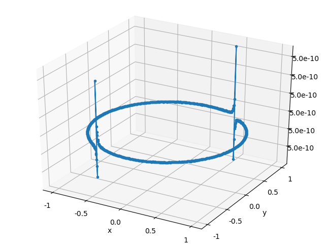
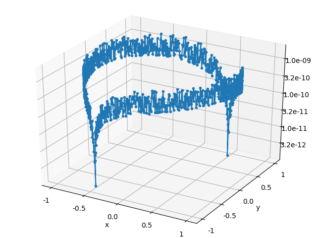
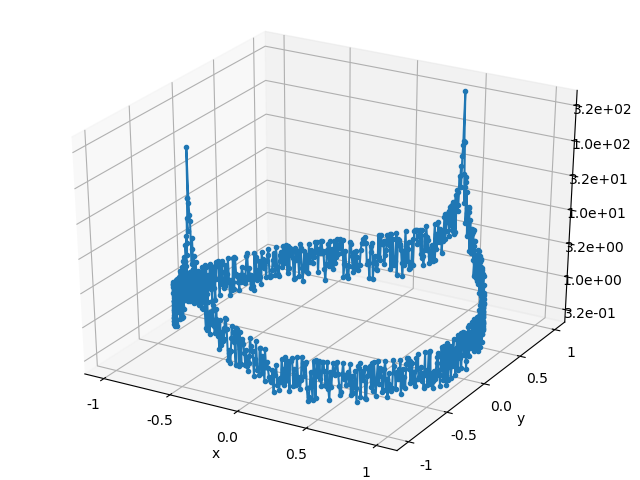
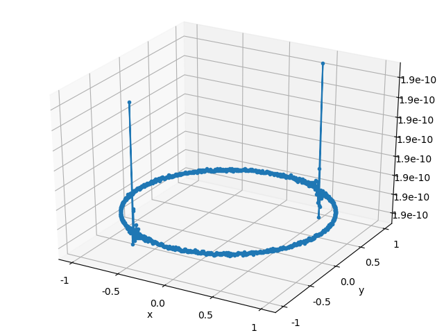
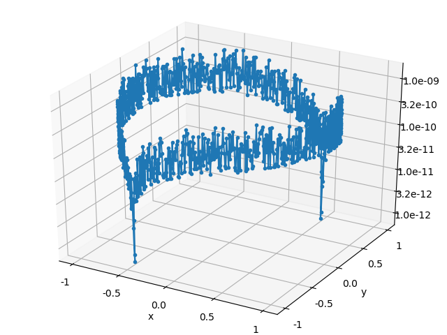
\] Plots of the solution relative error, backward error, and ratio of the errors are listed below for both of the solution algorithms. Each point in the error plots has the form \((b_1, b_2, \text{err})\), where \(b_1\) and \(b_2\) are the coordinates of the right hand side \(b\), and \(\text{err}\) is the type error indicated in the plot’s caption.

The relative error of the solution obeys the expected bound, but the plots of the backward error indicate that both algorithms typically compute a solution whose associated backward error is comparable in magnitude to the solution error. I didn’t expect the backward and forward error to have the same magnitude, so color me surprised. In part II, I’ll give a more detailed explanation of where the solution error enters into the calculation.

The code for the numerical experiments, and plot generation is on Github.

Gaussian elimination

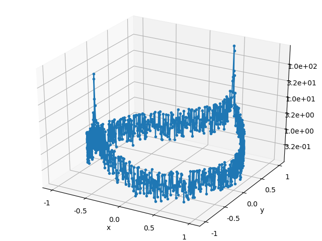
QR